1. Remove Subtotals in Pivot Table
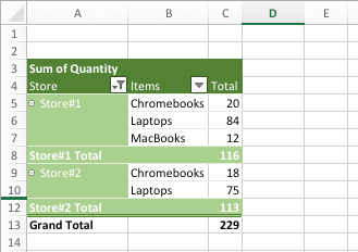
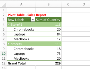
In the Pivot Table below, we have “Grand Total” for all the products sold and also the “Subtotals” for products sold by Store#1 and Store#2.
Since, we only have 2 stores, the subtotals look good and provide additional information. However, as you add more stores to the report, the number of subtotals will also grow and this may end up making the report look crowded. In such a case, you may find it necessary to get rid of the subtotals, in order to make your report look clean and easy to follow.
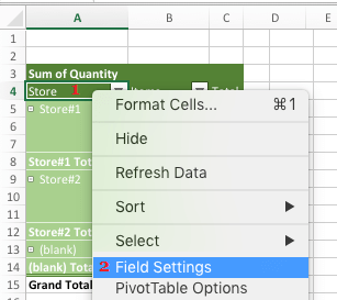
Right-click on the Store Entry and click on Field Settings option in the contextual menu that appears.
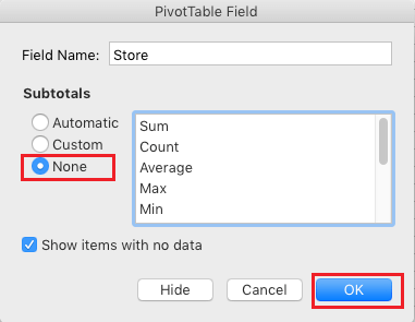
On the Field Data Settings screen, select the None option and click on the OK button.
This will remove the Subtotals for Store#1 and Store#2 and the Pivot Table will only indicate the Grand Total of items sold by both the stores.
2. Add Subtotals in Pivot Table
Depending on your requirements, you may find the need to show Subtotals in Pivot Table. In such a case, you can follow the steps below to Add Subtotals in Pivot Table.
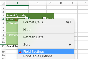
Right-click on the Store Entry and click on Field Settings option in the contextual menu.
On the next screen, select the Automatic option and click on OK to Add Subtotals in Pivot Table.
As you can see in the image above, adding subtotals in Pivot Table has made the report look more useful by providing both summary of items sold by each store and also the Grand Total of all the items sold.
How to Create Pivot Table From Multiple Worksheets How to Create Two Pivot Tables in Single Worksheet

